In the evaluation of new signals and trading strategies, a common practice is to initiate the research process by analyzing a full set of trade statistics. The rationale behind this approach is simple: strategies exhibiting attractive trade-level metrics are considered eligible for further due diligence, whereas those that do not can be quickly rejected.
While this approach may appear reasonable at first glance, our experience reveals that it can conceal a significant and potentially misleading bias.
We define the concept of opportunity-set bias as the gap between the expected performance implied by a full sample of trade-level statistics and the actual performance that can realistically be achieved. This bias arises when the analysis implicitly assumes that all observed trades in the dataset could have been executed: in reality, this is not always feasible.
Models that offer highly time-varying and clustered opportunity sets are particularly vulnerable to this bias: in such cases, trades often emerge in large, concentrated bursts, raising serious concerns about the ability to execute all of them given real-world execution and position management constraints. As a result, the theoretical performance inferred from the full trade set can substantially deviate from the performance that can be realistically captured.
In this article, through the case study of a simple mean-reversion signal, we provide empirical proof of this impactful yet often overlooked bias.
A Simple Mean Reversion Signal
Within the domain of mean-reversion strategies, one indicator continues to stand out for its enduring popularity: the 2-period RSI, originally introduced by Larry Connors and Cesar Alvarez in Short-Term Trading Strategies That Work (2008).
In this study, we analyze a sample of more than 100,000 trade outcomes generated by a canonical mean-reversion framework built around RSI(2), applied to all historical constituents of the S&P 500 from 1996 until November 2025.
The strategy rules are defined as follows:
- Entry: If a stock’s RSI(2) reading falls below 5 and its price closes below the 5-day moving average, initiate a long position at the next day’s open.
- Price Exit: Close the position at the next day’s open following the first close above the 5-day moving average.
- Time Exit: Force an exit at the next day’s open after holding the position for 5 trading days.
Such strategy has generated a total of 114,189 trades, with a mean return per trade of 45 bps and a hit-ratio of 64%.
Opportunity Set and Market Selloffs
Although we did expect this framework to produce a time-varying opportunity set, the magnitude of its variability was far greater than anticipated. On days when signals appeared, the median number of eligible trades was 9, with peaks occasionally above 50 and a maximum recorded value of 250.
What appears even more striking is the highly skewed distribution of trades across days. Our analysis indicates that a mere 3.1% of days are responsible for 50% of the whole trade set, with nearly all trading activity (95%) occurring within just one-third (32.6%) of the days on which the strategy was active.
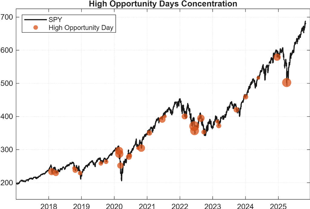
Figure 1. The plot highlights how high-opportunity days tend to cluster during S&P 500 sell-offs. Orange dots indicate days where more than 100 signals were identified.
Furthermore, a distinct pattern emerges when isolating “high-opportunity days” (defined as sessions generating at least 100 entry signals). As illustrated in Figure 1, the largest clusters of opportunities coincide with broad market selloffs. This is fully aligned with the mechanics of mean reversion: during market-wide declines, a substantial portion of the universe is simultaneously pushed into short-term oversold territory, triggering dozens—sometimes hundreds—of entry signals at once.
This dynamic reveals an important yet often overlooked issue in trade-level analyses. When practitioners compute performance metrics on the full sample of trades, they implicitly give the same statistical weight to each trade, regardless of the market state in which it occurred. But on high-opportunity days—typically driven by beta-dominated selloffs rather than idiosyncratic events—those trades tend to be both more profitable and highly correlated with one another. As a result, full-sample statistics become artificially inflated: these clustered, state-dependent trades dominate the dataset far more than they could ever dominate real-world PnL.
Seen through this lens, the standard assumption that all observed trades could have been executed becomes very difficult to justify. How can one realistically deploy capital in a framework where the opportunity set can surge from 5 trades to 100 from one day to the next? Once leverage limits are reached, accommodating a sudden influx of signals would require scaling down or liquidating existing positions, driving turnover and transaction costs sharply higher and eroding the strategy’s expected performance.
The Opportunity Set Bias
One way to address this issue is to explicitly incorporate position constraints into the trade analysis process: this can be achieved through the use of a bootstrapping procedure.
In our study, we model a capacity-constrained environment by running 10,000 simulations in which, on each day, at most five trades can be executed, with each trade randomly selected from that day’s pool of eligible signals. We can also think of this as generating 10,000 different sub-tables from our full-sized trades dataset, with a maximum of 5 trades randomly picked within each day.
This approach allows us to approximate the distribution of trade returns that a practitioner could more realistically capture, and to quantify the potential performance loss (or gain) relative to the unconstrained full-sample benchmark.
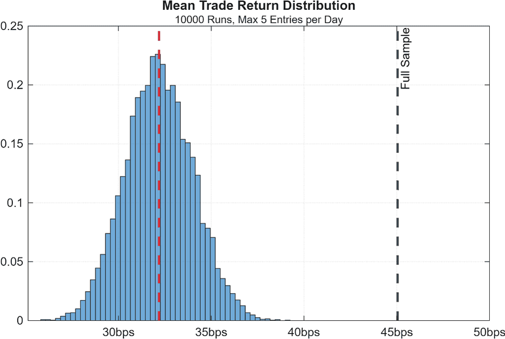
Figure 2. Distribution of mean trade returns across 10,000 simulations of a capacity-constrained version of a mean-reversion trading system
The results reveal a clear inefficiency: even the top-performing simulations fail to match the mean trade return obtained when executing across the full universe of daily signals. In the context of our strategy, this divergence is what we refer to as the opportunity-set bias.
In other words, rather profitable trades appear frequently over our full sample, but in such a clustered way that makes it unrealistic to capture them all. Real-life operational limits force us to discard most of those highly profitable (yet extremely clustered) signals, and this drastically reduces their contribution to our mean trade return metric.
To illustrate this dynamic with a simple example, imagine a dataset of trade-level statistics across 100 days:
- Half the days have a single trade with a -1% loss.
- The other half have 10 trades, each returning +1%.
Without position constraints, the mean trade return appears to be largely profitable, as the sheer volume of positive trades drowns out the losers. Instead, under a restrictive cap of maximum one trade per day, the volume advantage disappears: we would be left with an equal number of winning and losing trades, resulting in a strategy with an expected return of 0%. Even though this example is deliberately extreme, it precisely captures what is happening in our real dataset.
This return-clustering phenomenon can also be visualized by ranking the full sample of trade returns from best to worst and grouping them into twenty equal-sized buckets (i.e. vigintiles). For each bucket, we calculate the average opportunity set size present on the days when those trades were executed, and what we observe is a skewed U-shaped pattern.
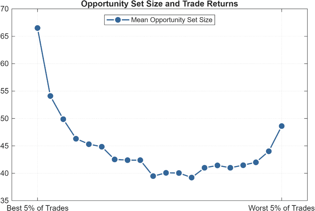
Figure 3. Visual representation of the opportunity-clustering phenomenon. Individual trades are ranked by their return and segmented into vigintiles. Y-axis is the mean daily opportunity set size for each bucket.
We clearly see that the most profitable 5% of all trades take place when the daily opportunity set amounts to ≈65 signals: by limiting ourselves to selecting only 5 trades, we can gain exposure to less than 8% of all the available opportunities on those days.
Key Takeaways
Evaluating a trading signal purely through full-sample trade statistics can be dangerously misleading whenever the strategy exhibits time-varying and clustered opportunity sets. In such cases, the implicit assumption that all observed trades could have been executed does not hold in practice.
Our analysis shows that:
1. The most profitable trades occur on the same days when the opportunity set explodes.
These periods typically coincide with broad market selloffs, when a large fraction of the universe simultaneously meets the oversold criteria. Since only a limited number of positions can be initiated on those days, the majority of these highly profitable signals are unavoidably missed.
2. Full-sample statistics overweight rare, high-opportunity regimes.
The mean return of the “unconstrained” trade set gives disproportionate weight to a handful of crisis-like days that are rich in opportunities but impossible to fully exploit. This creates an upward bias in trade-level return estimates.
3. Capacity and position constraints fundamentally reshape expected performance.
Even simple constraints—such as limiting executions to five trades per day—materially reduce both return and Sharpe potential. In our bootstrap experiment, none of the 10,000 feasible simulations matched the full-sample mean return, highlighting a structural inefficiency induced by clustering.
4. Return distributions are state-dependent, not IID.
The vigintile analysis reveals a U-shaped pattern: both the best and worst trades occur in high-clustering environments. This confirms that trade profitability is tightly linked to market state, invalidating the assumption that each trade is an independent outcome drawn from the same distribution.
5. Opportunity-set bias is an invisible but powerful distortion.
It does not manifest through slippage or transaction costs—rather, it arises because the strategy systematically produces more signals in environments that cannot be traded at full capacity. As a consequence, theoretical alpha decays when translated into a realistic portfolio-level framework.
What This Means in Practice
Whenever a strategy displays opportunity spikes:
- Do not rely on full-sample trade statistics.
- Incorporate capacity constraints early in the research process.
- Evaluate how signals behave during high-opportunity days.
- Model realistic throughput using random or ranked subsampling.
- Focus research efforts on identifying which signals to prioritize on those crowded days.
Ignoring these dynamics often leads to overly optimistic backtests, miscalibrated expectations, and strategies that fail to survive real deployment.