Designing a Profitable Intraday Strategy Using Python and Alpaca
In this article, we provide the Python code required to backtest a profitable intraday strategy on SPY. This strategy not only exploits the trading edge presented in our paper, ‘Beat the Market: An Effective Intraday Momentum Strategy for the S&P500 ETF (SPY),’ but it also takes advantage of overnight gaps that typically revert within the first 30 minutes of the trading session.
Furthermore, for this backtest, we use Alpaca as our data provider because it offers 8 years of free intraday data for many US stocks and ETFs. This is a significant improvement, considering that Polygon offers only 2 years of free data.
In this blog post, we build upon the Python code that was translated from MATLAB, as initially presented in our previous article where we backtested two years of free data. Our aim is to make the code more accessible and intuitive, especially for novice quantitative researchers. To enhance readability, we have intentionally avoided complex coding procedures that could increase computational efficiency but might obscure understanding. This updated version extends the backtesting period to over seven years and introduces an overnight gap reversal signaling strategy, enhancing both the scope and depth of our analysis.
Step-by-Step Guide Through the Backtesting Process
Below, we give an overview of the main building blocks behind the backtesting procedure.
Step 2: Add Key Variables – We explain how to calculate key indicators presented in the paper, such as VWAP, Move (from Open), Sigma_Open, SPY Rolling Volatility, and many others. These indicators are required to run the backtest of the strategy.
Step 3: Backtesting – Dive into the actual backtesting process; create the main time series needed to conduct statistical inferences and performance evaluation.
Step 4: Study Results – We show how to plot the equity line of the trading strategy in conjunction with the passive Buy & Hold portfolio. Learn how to use historical returns time series to evaluate the profitability and risk behind the intraday momentum strategy.
Tools Needed
Python: Python is a versatile programming language widely used for data analysis and visualization. It’s free and open-source.
Pandas: Pandas is a Python library for data manipulation and analysis, ideal for working with numerical tables and time series.
Matplotlib: Matplotlib is a Python library for creating a wide variety of static, animated, and interactive visualizations.
Statsmodels: Statsmodels provides tools for statistical modeling in Python, offering numerous methods for regression and time series analysis.
How to Read This Post
For each step, we will provide the full code first, then explain it step by step. If a step depends on a utility function (a function we wrote that is not built-in Python), we will provide its code after the step code directly before the explanation.
We recommend opening the following Google Colab Notebook and follow explanations in this article when needed.
In this step, we utilize Alpaca’s API to fetch intraday, daily, and dividend data for the SPY ETF. Even though Alpaca provides many financial time series for each ticker, for the sake of our backtest, we only need historical data for OHLC (open, high, low, close), Volume, Time, and Dividends.
Click to see the Python code for fetch_alpaca_data & fetch_alpaca_dividends
Python
API_KEY_ID = "API_KEY_ID"API_SECRET_KEY = "API_SECRET_KEY"deffetch_alpaca_data(symbol, timeframe, start_date, end_date):""" Fetch stock bars data from Alpaca Markets based on the given timeframe. """ url = 'https://data.alpaca.markets/v2/stocks/bars' headers = {'APCA-API-KEY-ID': API_KEY_ID,'APCA-API-SECRET-KEY': API_SECRET_KEY } params = {'symbols': symbol,'timeframe': timeframe,'start': datetime.strptime(start_date, "%Y-%m-%d").isoformat() + 'Z','end': datetime.strptime(end_date, "%Y-%m-%d").isoformat() + 'Z','limit': 10000,'adjustment': 'raw','feed': 'sip' } data_list = [] eastern = pytz.timezone('America/New_York') utc = pytz.utc market_open = time(9, 30) # Market opens at 9:30 AM market_close = time(15, 59) # Market closes just before 4:00 PMprint("Starting data fetch...")whileTrue:print(f"Fetching data for symbols: {symbol} from {start_date} to {end_date}") response = requests.get(url, headers=headers, params=params)if response.status_code != 200:print(f"Error fetching data with status code {response.status_code}: {response.text}")break data = response.json() bars = data.get('bars')for symbol, entries in bars.items():print(f"Processing {len(entries)} entries for symbol: {symbol}")for entry in entries:try: utc_time = datetime.fromisoformat(entry['t'].rstrip('Z')).replace(tzinfo=utc) eastern_time = utc_time.astimezone(eastern)# Apply market hours filter for '1Min' timeframeif timeframe == '1Min'andnot (market_open <= eastern_time.time() <= market_close):continue# Skip entries outside market hours data_entry = {'volume': entry['v'],'open': entry['o'],'high': entry['h'],'low': entry['l'],'close': entry['c'],'caldt': eastern_time } data_list.append(data_entry)print(f"Appended data for {symbol} at {eastern_time}")exceptExceptionas e:print(f"Error processing entry: {entry}, {e}")continueif'next_page_token'in data and data['next_page_token']: params['page_token'] = data['next_page_token']print("Fetching next page...")else:print("No more pages to fetch.")break df = pd.DataFrame(data_list)print("Data fetching complete.")return dfdeffetch_alpaca_dividends(symbol, start_date, end_date):""" Fetch dividend announcements from Alpaca for a specified symbol between two dates. This function splits the request into manageable 90-day segments to comply with API constraints. """ url_base = "https://paper-api.alpaca.markets/v2/corporate_actions/announcements" headers = {"accept": "application/json","APCA-API-KEY-ID": API_KEY_ID,"APCA-API-SECRET-KEY": API_SECRET_KEY } start_date = datetime.strptime(start_date, "%Y-%m-%d").date() end_date = datetime.strptime(end_date, "%Y-%m-%d").date() dividends_list = [] current_start = start_datewhile current_start < end_date: current_end = min(current_start + timedelta(days=89), end_date) url = f"{url_base}?ca_types=Dividend&since={current_start}&until={current_end}&symbol={symbol}" response = requests.get(url, headers=headers)if response.status_code == 200: data = response.json()for entry in data: dividends_list.append({'caldt': datetime.strptime(entry['ex_date'], '%Y-%m-%d'),'dividend': float(entry['cash']) })else:print(f"Failed to fetch data for period {current_start} to {current_end}: {response.text}") current_start = current_end + timedelta(days=1)return pd.DataFrame(dividends_list)
Explanation:
To initiate the backtest, we require high-quality intraday trading data. Here, we use Alpaca’s API, a reliable source for financial data that provides access to intraday data for FREE starting from 2016. This example demonstrates how to fetch this data using custom Python functions that adjust the timestamp from UTC to NY Market time (from 9:30 AM to 3:59 PM) and filter for market hours only.
After running the codes, the data frames will have the following:
spy_intra_data: Includes intraday volume and OHLC (open, high, low, close).
spy_daily_data: Contains daily volume and OHLC.
dividends: Stores dividend dates and amounts.
You must obtain a free API Key by registering with Alpaca. Consider securely managing your API key, such as using a virtual environment variable for sensitive information.
When you receive your API Key, remember to update lines 1 and 2 in the code snippet with the actual API Key values, ensuring they are enclosed in quotes, like “EXAMPLE_API_KEY” and not EXAMPLE_API_KEY. If it’s not clear how to do this, a video on our Twitter page will provide a demonstration.
Step 2: Add Key Variables
Overview
In this step, we’ll dive into the calculations of various technical indicators that are crucial for running the backtest in Step 3. These metrics include VWAP, Move (from Open), Sigma_Open, SPY Rolling Volatility, and many others. Each step is broken down for clarity.
Step 2 Code:
Click to see the Python Code for Step 2
Python
# Load the intraday data into a DataFrame and set the datetime column as the index.df = pd.DataFrame(spy_intra_data)df['day'] = pd.to_datetime(df['caldt']).dt.date # Extract the date part from the datetime for daily analysis.df.set_index('caldt', inplace=True) # Setting the datetime as the index for easier time series manipulation.# Group the DataFrame by the 'day' column to facilitate operations that need daily aggregation.daily_groups = df.groupby('day')# Extract unique days from the dataset to iterate through each day for processing.all_days = df['day'].unique()# Initialize new columns to store calculated metrics, starting with NaN for absence of initial values.df['move_open'] = np.nan # To record the absolute daily change from the open pricedf['vwap'] = np.nan # To calculate the Volume Weighted Average Price.df['spy_dvol'] = np.nan # To record SPY's daily volatility.# Create a series to hold computed daily returns for SPY, initialized with NaN.spy_ret = pd.Series(index=all_days, dtype=float)# Iterate through each day to calculate metrics.for d inrange(1, len(all_days)): current_day = all_days[d] prev_day = all_days[d - 1]# Access the data for the current and previous days using their groups. current_day_data = daily_groups.get_group(current_day) prev_day_data = daily_groups.get_group(prev_day)# Calculate the average of high, low, and close prices. hlc = (current_day_data['high'] + current_day_data['low'] + current_day_data['close']) / 3# Compute volume-weighted metrics for VWAP calculation. vol_x_hlc = current_day_data['volume'] * hlc cum_vol_x_hlc = vol_x_hlc.cumsum() # Cumulative sum for VWAP calculation. cum_volume = current_day_data['volume'].cumsum()# Assign the calculated VWAP to the corresponding index in the DataFrame. df.loc[current_day_data.index, 'vwap'] = cum_vol_x_hlc / cum_volume# Calculate the absolute percentage change from the day's opening price. open_price = current_day_data['open'].iloc[0] df.loc[current_day_data.index, 'move_open'] = (current_day_data['close'] / open_price - 1).abs()# Compute the daily return for SPY using the closing prices from the current and previous day. spy_ret.loc[current_day] = current_day_data['close'].iloc[-1] / prev_day_data['close'].iloc[-1] - 1# Calculate the 15-day rolling volatility, starting calculation after accumulating 15 days of data.if d > 14: df.loc[current_day_data.index, 'spy_dvol'] = spy_ret.iloc[d - 15:d-1].std(skipna=False)# Calculate the minutes from market open and determine the minute of the day for each timestamp.df['min_from_open'] = ((df.index - df.index.normalize()) / pd.Timedelta(minutes=1)) - (9 * 60 + 30) + 1df['minute_of_day'] = df['min_from_open'].round().astype(int)# Group data by 'minute_of_day' for minute-level calculations.minute_groups = df.groupby('minute_of_day')# Calculate rolling mean and delayed sigma for each minute of the trading day.df['move_open_rolling_mean'] = minute_groups['move_open'].transform(lambdax: x.rolling(window=14, min_periods=13).mean())df['sigma_open'] = minute_groups['move_open_rolling_mean'].transform(lambdax: x.shift(1))# Convert dividend dates to datetime and merge dividend data based on trading days.dividends['day'] = pd.to_datetime(dividends['caldt']).dt.datedf = df.merge(dividends[['day', 'dividend']], on='day', how='left')df['dividend'] = df['dividend'].fillna(0) # Fill missing dividend data with 0.
Explanation:
2.1 Preparing Data Variables
Date and Time Variables:
df[‘day’]: This represents the trading day by converting the caldt datetime column into just the date component, effectively separating the date from time.
Click to see the Python Code
Python
df['day'] = pd.to_datetime(df['caldt']).dt.date
Index Setting:
df.set_index(‘caldt’): This sets the caldtcolumn as the DataFrame’s index, facilitating efficient time-series operations and enabling easier slicing and access based on time.
Click to see the Python Code
Python
df.set_index('caldt', inplace=True)
2.2 Grouping and Data Aggregation
Daily Grouping for Efficient Access:
Group Data by Day: This organizes the data into groups based on each unique trading day, facilitating easier daily aggregations and calculations.
Click to see the Python Code
Python
daily_groups = df.groupby('day')
Unique Days Extraction:
Extract Unique Trading Days: Retrieves all unique days from the data, providing a basis for day-by-day iterations in subsequent calculations.
Click to see the Python Code
Python
all_days = df['day'].unique()
2.3 Initializing Variables for Metrics
Metric Placeholders Initialization:
NaN Initialization: Columns such as move_open, vwap, and spy_dvolare initialized with NaN values, setting up placeholders for calculated trading metrics.
Click to see the Python Code
Python
df['move_open'] = np.nan # To record the absolute daily change from the open pricedf['vwap'] = np.nan # To calculate the Volume Weighted Average Price.df['spy_dvol'] = np.nan # To record SPY's daily volatility.
Daily Returns and Volatility Preparation:
spy_ret Series: Sets up a Pandas Series to capture computed daily returns for SPY, initialized with NaN to accommodate future numerical operations.
Click to see the Python Code
Python
spy_ret = pd.Series(index=all_days, dtype=float)
2.4 Computation of Daily Metrics
Daily Metrics Calculation Loop: This loop calculates various metrics for each day by iterating through all unique trading days
VWAP Calculation: Computes the Volume Weighted Average Price using cumulative sums of volume times the average of high, low, and close prices.
Open Price Movement: Calculates the absolute percentage change from the day’s opening price to the close.
Daily Returns: Computes the daily return for SPY using the close prices of the current and previous days.
Rolling Volatility: Calculates a 15-day rolling volatility of SPY returns, starting calculations after at least 14 days of data are available.
Click to see the Python Code
Python
# Iterate through each day to calculate metrics.for d inrange(1, len(all_days)): current_day = all_days[d] prev_day = all_days[d - 1]# Access the data for the current and previous days using their groups. current_day_data = daily_groups.get_group(current_day) prev_day_data = daily_groups.get_group(prev_day)# Calculate the average of high, low, and close prices. hlc = (current_day_data['high'] + current_day_data['low'] + current_day_data['close']) / 3# Compute volume-weighted metrics for VWAP calculation. vol_x_hlc = current_day_data['volume'] * hlc cum_vol_x_hlc = vol_x_hlc.cumsum() # Cumulative sum for VWAP calculation. cum_volume = current_day_data['volume'].cumsum()# Assign the calculated VWAP to the corresponding index in the DataFrame. df.loc[current_day_data.index, 'vwap'] = cum_vol_x_hlc / cum_volume# Calculate the absolute percentage change from the day's opening price. open_price = current_day_data['open'].iloc[0] df.loc[current_day_data.index, 'move_open'] = (current_day_data['close'] / open_price - 1).abs()# Compute the daily return for SPY using the closing prices from the current and previous day. spy_ret.loc[current_day] = current_day_data['close'].iloc[-1] / prev_day_data['close'].iloc[-1] - 1# Calculate the 15-day rolling volatility, starting calculation after accumulating 15 days of data.if d > 14: df.loc[current_day_data.index, 'spy_dvol'] = spy_ret.iloc[d - 15:d-1].std(skipna=False)
2.5 Minute-level Calculations:
Minute from Market Open:
Calculates the minutes from market open for each timestamp, helping in analyzing intraday trends and movements.
Rolling Mean and Delayed Sigma Calculations:
Calculates rolling means and a shifted sigma (standard deviation) for opening movements, to explore more nuanced intraday dynamics.
Converts dividend dates to datetime and merges this data based on trading days, accounting for dividends in the analysis which is crucial for accurate return calculations.
Now that we have our needed Indicators, lets start backtesting!
Step 3: Backtesting
Overview
In this part, we conduct the actual backtest. This section involves defining the trading environment, including assets under management (AUM), commission costs, maximum leverage, volatility multiplier, and many others. To improve the readability of the code, we used a for loop where each iteration represents a historical trading day.
Step 3 Code:
Click to see the Python Code for Step 3
Python
# Constants and settingsAUM_0 = 100000.0commission = 0.0035min_comm_per_order = 0.35band_mult = 1trade_freq = 30sizing_type = "vol_target"target_vol = 0.02max_leverage = 4overnight_threshold = 0.02# Group data by day for faster accessdaily_groups = df.groupby('day')# Initialize strategy DataFrame using unique daysstrat = pd.DataFrame(index=all_days)strat['ret'] = np.nanstrat['AUM'] = AUM_0strat['ret_spy'] = np.nan# Calculate daily returns for SPY using the closing pricesdf_daily = pd.DataFrame(spy_daily_data)df_daily['caldt'] = pd.to_datetime(df_daily['caldt']).dt.datedf_daily.set_index('caldt', inplace=True) # Set the datetime column as the DataFrame index for easy time series manipulation.df_daily['ret'] = df_daily['close'].diff() / df_daily['close'].shift()# Loop through all days, starting from the second dayfor d inrange(1, len(all_days)): current_day = all_days[d] prev_day = all_days[d-1]if prev_day in daily_groups.groups and current_day in daily_groups.groups: prev_day_data = daily_groups.get_group(prev_day) current_day_data = daily_groups.get_group(current_day)if'sigma_open'in current_day_data.columns and current_day_data['sigma_open'].isna().all():continue prev_close_adjusted = prev_day_data['close'].iloc[-1] - df.loc[current_day_data.index, 'dividend'].iloc[-1] open_price = current_day_data['open'].iloc[0] current_close_prices = current_day_data['close'] spx_vol = current_day_data['spy_dvol'].iloc[0] vwap = current_day_data['vwap'] sigma_open = current_day_data['sigma_open'] UB = max(open_price, prev_close_adjusted) * (1 + band_mult * sigma_open) LB = min(open_price, prev_close_adjusted) * (1 - band_mult * sigma_open)# Determine trading signals signals = np.zeros_like(current_close_prices) signals[(current_close_prices > UB) & (current_close_prices > vwap)] = 1 signals[(current_close_prices < LB) & (current_close_prices < vwap)] = -1# Position sizing previous_aum = strat.loc[prev_day, 'AUM']if sizing_type == "vol_target":if math.isnan(spx_vol): shares = round(previous_aum / open_price * max_leverage)else: shares = round(previous_aum / open_price * min(target_vol / spx_vol, max_leverage))elif sizing_type == "full_notional": shares = round(previous_aum / open_price)# Apply trading signals at trade frequencies trade_indices = np.where(current_day_data["min_from_open"] % trade_freq == 0)[0] exposure = np.full(len(current_day_data), np.nan) # Start with NaNs exposure[trade_indices] = signals[trade_indices] # Apply signals at trade times# Custom forward-fill that stops at zeros last_valid = np.nan # Initialize last valid value as NaN filled_values = [] # List to hold the forward-filled valuesfor value in exposure:ifnot np.isnan(value): # If current value is not NaN, update last valid value last_valid = valueif last_valid == 0: # Reset if last valid value is zero last_valid = np.nan filled_values.append(last_valid) exposure = pd.Series(filled_values, index=current_day_data.index).shift(1).fillna(0).values # Calculate trades count based on changes in exposure trades_count = np.sum(np.abs(np.diff(np.append(exposure, 0)))) overnight_move = (open_price / prev_close_adjusted - 1) open_trade_signal = -np.sign(overnight_move) * (abs(overnight_move) > overnight_threshold) trade_time_row = current_day_data[current_day_data['min_from_open'] == trade_freq] exit_price_minute_version_trade = trade_time_row['close'].iloc[0]# Calculate PnL of Mean-Reversion Portfolio (MRP) pnl_mean_reversion_trade = open_trade_signal * shares * (exit_price_minute_version_trade - open_price) comm_mean_reversion_trade = 2 * max(min_comm_per_order, commission * shares) * abs(open_trade_signal) net_pnl_mean_reversion = pnl_mean_reversion_trade - comm_mean_reversion_trade# Calculate PnL of Intraday Momentum Portfolio (IMP) change_1m = current_close_prices.diff() gross_pnl = np.sum(exposure * change_1m) * shares commission_paid = trades_count * max(min_comm_per_order, commission * shares) net_pnl_mom = gross_pnl - commission_paid# Calculate Total PNL net_pnl = net_pnl_mom + net_pnl_mean_reversion# Update the daily return and new AUM strat.loc[current_day, 'AUM'] = previous_aum + net_pnl strat.loc[current_day, 'ret'] = net_pnl / previous_aum# Save the passive Buy&Hold daily return for SPY strat.loc[current_day, 'ret_spy'] = df_daily.loc[df_daily.index == current_day, 'ret'].values[0]
Explanation:
3.1 Initial Setup and Parameters
Set the initial parameters required for the backtest:
Prepare the data and initialize the strategy Data Frame:
Click to see the Python Code
Python
# Group data by day for faster accessdaily_groups = df.groupby('day')# Initialize strategy DataFrame using unique daysstrat = pd.DataFrame(index=all_days)strat['ret'] = np.nanstrat['AUM'] = AUM_0strat['ret_spy'] = np.nan
3.3 Calculate Daily Returns for SPY
Calculate and set the daily returns for SPY based on the close prices, this will be used for benchmarking (BUY&HOLD) :
Loop through each trading day and access the necessary data:
Click to see the Python Code
Python
for d inrange(1, len(all_days)): current_day = all_days[d] prev_day = all_days[d-1]if prev_day in daily_groups.groups and current_day in daily_groups.groups: prev_day_data = daily_groups.get_group(prev_day) current_day_data = daily_groups.get_group(current_day)if'sigma_open'in current_day_data.columns and current_day_data['sigma_open'].isna().all():continue# Skip if no valid sigma data
3.5 Position Sizing and Trading Signals
Determine the position size and calculate trading signals:
3.9 Aggregate the PnL from Intraday Momentum Portfolio and Mean-Reversion Portfolio
Consolidate the daily profit and loss from both the Intraday Momentum Portfolio (IMP) and the Mean-Reversion Portfolio (MRP)
Click to see the Python Code
Python
# Calculate the aggregate daily PnL summing the PnL of MRP and PnL of IMPnet_pnl = net_pnl_mom + net_pnl_mean_reversion
3.10 Record Passive Buy&Hold and Active Strategy Returns
Record the passive Buy&Hold returns along with updates for daily returns and assets under management (AUM) for comparison
Click to see the Python Code
Python
# Update the daily return and new AUMstrat.loc[current_day, 'AUM'] = previous_aum + net_pnlstrat.loc[current_day, 'ret'] = net_pnl / previous_aum# Save the passive Buy&Hold daily return for SPYstrat.loc[current_day, 'ret_spy'] = df_daily.loc[df_daily.index == current_day, 'ret'].values[0]
And that’s it, our backtesting is done! lets see the results in the next step.
Step 4: Study Results
Overview
In this step, we analyze the results of the trading strategy by visualizing the growth of Assets Under Management (AUM) over time for both the strategy and a passive investment in the S&P 500. Additionally, we compute various performance metrics to assess the strategy’s effectiveness.
Step 4 Code:
Click to see the Python Code
Python
# Calculate cumulative products for AUM calculationsstrat['AUM_SPX'] = AUM_0 * (1 + strat['ret_spy']).cumprod(skipna=True)# Create a figure and a set of subplotsfig, ax = plt.subplots()# Plotting the AUM of the strategy and the passive S&P 500 exposureax.plot(strat.index, strat['AUM'], label='Momentum', linewidth=2, color='k')ax.plot(strat.index, strat['AUM_SPX'], label='S&P 500', linewidth=1, color='r')# Formatting the plotax.grid(True, linestyle=':')ax.xaxis.set_major_locator(mdates.MonthLocator())ax.xaxis.set_major_formatter(mdates.DateFormatter('%b %y'))plt.xticks(rotation=90)ax.yaxis.set_major_formatter(FuncFormatter(lambdax, _: f'${x:,.0f}'))ax.set_ylabel('AUM ($)')plt.legend(loc='upper left')plt.title('Intraday Momentum Strategy', fontsize=12, fontweight='bold')plt.suptitle(f'Commission = ${commission}/share', fontsize=9, verticalalignment='top')# Show the plotplt.show()# Calculate additional stats and display themstats = {'Total Return (%)': round((np.prod(1 + strat['ret'].dropna()) - 1) * 100, 0),'Annualized Return (%)': round((np.prod(1 + strat['ret']) ** (252 / len(strat['ret'])) - 1) * 100, 1),'Annualized Volatility (%)': round(strat['ret'].dropna().std() * np.sqrt(252) * 100, 1),'Sharpe Ratio': round(strat['ret'].dropna().mean() / strat['ret'].dropna().std() * np.sqrt(252), 2),'Hit Ratio (%)': round((strat['ret'] > 0).sum() / (strat['ret'].abs() > 0).sum() * 100, 0),'Maximum Drawdown (%)': round(strat['AUM'].div(strat['AUM'].cummax()).sub(1).min() * -100, 0)}Y = strat['ret'].dropna()X = sm.add_constant(strat['ret_spy'].dropna())model = sm.OLS(Y, X).fit()stats['Alpha (%)'] = round(model.params.const * 100 * 252, 2)stats['Beta'] = round(model.params['ret_spy'], 2)print(stats)
4.1 AUM Calculation for Active and Passive S&P 500 Exposure
Compute the cumulative product of the returns, which represents the growth of the initial investment (AUM) over time.
Click to see the Python Code
Python
# Calculate the cumulative AUM for the strategy and S&P 500strat['AUM_SPX'] = AUM_0 * (1 + strat['ret_spy']).cumprod(skipna=True)
4.2 Plotting AUM
Use matplotlibto create a plot that shows how the AUM
Click to see the Python Code
Python
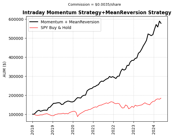
# Create a figure and a set of subplotsfig, ax = plt.subplots()# Plotting the AUM of the strategy and the passive S&P 500 exposureax.plot(strat.index[::20], strat['AUM'].iloc[::20], label='Momentum + MeanReversion', linewidth=2, color='k')ax.plot(strat.index[::20], strat['AUM_SPX'].iloc[::20], label=f'{symbol} Buy & Hold', linewidth=1, color='r')# Formatting the plotax.grid(True, linestyle=':')ax.xaxis.set_major_locator(mdates.YearLocator())ax.xaxis.set_major_formatter(mdates.DateFormatter('%Y'))plt.xticks(rotation=90)ax.set_ylabel('AUM ($)')plt.legend(loc='upper left')plt.title('Intraday Momentum Strategy+MeanReversion Strategy', fontsize=12, fontweight='bold')plt.suptitle(f'Commission = ${commission}/share', fontsize=9, verticalalignment='top')# Show the plotplt.show()
4.3 Calculate Additional Statistics
Compute various statistics to evaluate the performance of the trading strategy in comparison to a passive investment. These include total return, annualized return, volatility, Sharpe ratio, hit rate, maximum drawdown, and regression analysis for alpha and beta.
Regression analysis to determine the strategy’s alpha (performance relative to a benchmark) and beta (quantifies the sensitivity of an asset’s returns to the movements of the overall market).
Click to see the Python Code
Python
# Prepare data for regressionY = strat['ret'].dropna()X = sm.add_constant(strat['ret_spy'].dropna())# Conduct linear regressionmodel = sm.OLS(Y, X).fit()# Extract alpha and beta from the regression resultsstats['Alpha (%)'] = round(model.params.const * 100 * 252, 2)stats['Beta'] = round(model.params['ret_spy'], 2)
Results
Total Return (%): 472.0,
Annualized Return (%): 31.3,
Annualized Volatility (%): 14.6,
Sharpe Ratio: 1.95,
Hit Rate (%): 48.0,
Maximum Drawdown (%): 10.0,
Alpha (%): 29.43,
Beta: -0.08
Final Words
If you have questions or Ideas feel free to contact us on twitter/X or contact us directly here
"An object in motion tends to stay in motion, an object at rest tends to stay at rest."
Drawing on the principles first articulated by Isaac Newton in 1687, we are excited to announce the release of our new paper,