In short-term equity strategies, the delay between when a signal is computed and when it is executed can materially reduce performance. As shown in our research note When Execution Delays Erode Short-Term Alpha, computing a signal at the market close and executing it at the next morning open can remove a large portion of short-term alpha. Computing signals shortly before the close and executing them with Market on Close orders can preserve more of the intended edge while maintaining realistic backtesting assumptions.
The figure below illustrates this effect. A theoretical version that computes and executes at the close produces the highest cumulative return. Computing the signal at 15:45 ET and executing at the close tracks the theoretical result much more closely than the classic workflow of computing at the close and executing at the next open. The difference in long-term performance highlights why execution timing matters.
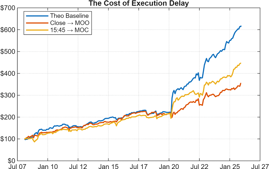
To enable this comparison historically, the database presented in this article captures both full-session daily prices and intraday prices up to 15:45 ET. The full-session daily prices reflect actual traded levels used in execution, and the 15:45 data represents what information would have been available before the close.
By preserving both views of the market, researchers can evaluate how much alpha survives when signals are formed before the close and executed at the official closing price, and how much is lost when execution is pushed to the next trading day. This structure makes it possible to backtest and compare realistic execution workflows with confidence.
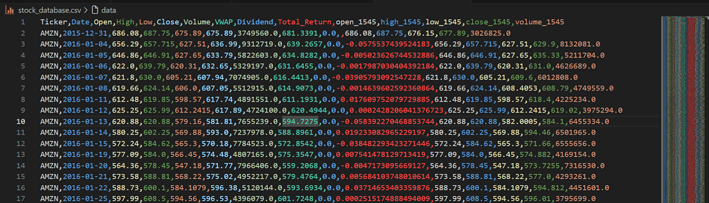
An Example of output using this workflow
Use-case: near-close signals
This dataset gives you both full-session daily OHLC and
intraday OHLCV aggregated to 15:45 ET.
You can test whether signals formed using
info available ~15min before the close
perform differently from waiting until the 16:00 auction.
For context on why timing matters for short-term alpha decay, see our research note
When Execution Delays Erode Short-Term Alpha.
Massive.com Stock Database Builder (Google Colab)
by Mohamed Gabriel, Software Engineer – Concretum Group
This notebook downloads multiple endpoints from Massive.com and builds a unified
total-return stock database. It includes unadjusted OHLC prices, split-adjusted closes,
dividends, and intraday bars covering the regular session
(15:30 timestamp captures [15:30, 15:45)).
No local setup required — runs entirely in your browser.
Previous usage
We previously used Massive.com (formerly Polygon.io) in earlier backtests, including an intraday momentum test on SPY and an opening-range breakout study. In this article, we shift the focus toward building a dataset suitable for total-return analysis and near-close execution testing.
Why We Use Multiple Data Representations
This process uses two Massive.com endpoints: one for aggregate price bars and one for dividends.
The price endpoint supports multiple representations via parameters (daily vs intraday, adjusted vs unadjusted), and each representation plays a specific role when constructing reinvested total return and evaluating near-close signals.
| API endpoint & config | Dataset | What it represents | Why we need it |
/v2/aggsday, adjusted=false | Daily Unadjusted Data | raw traded OHLC values | execution prices must match real historical levels |
/v2/aggsday, adjusted=true | Daily Adjusted Data | prices adjusted for stock splits | stable return denominator; avoids artificial price jumps |
/v3/reference/dividends
| Dividend Events | ex-dates and cash distributions | required for reinvested total return |
/v2/aggs15-minute, adjusted=false | Intraday 15-Minute Data | regular-session bars; last bar (15:30) gives prices available ~15min before 16:00 | test whether near-close signals perform differently from 16:00 execution |
Key Point
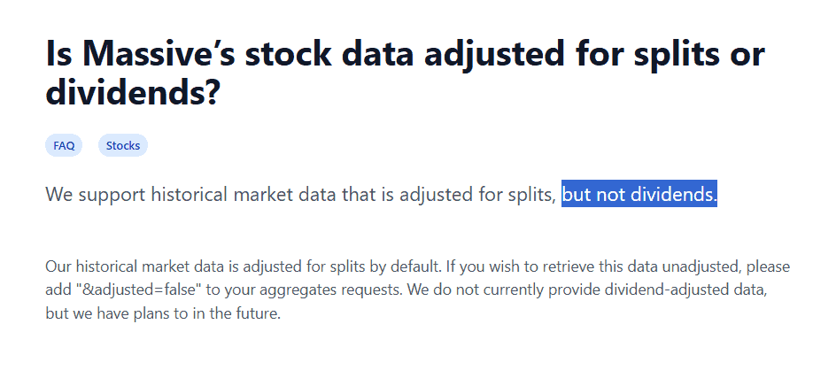
Total return is not the same as adjusted return.
Split-adjusted prices remove the effect of splits, but do not include dividends.
Cash dividends must be added to compute reinvested total return.
where:
\(C_t\) split-adjusted close at time t
\(C_{t-1}\) split-adjusted close one period earlier
\(D_t\) cash dividend paid at time t
What This Article Covers
This tutorial walks through downloading data from Massive.com, using different configurations of the aggregate price endpoint plus dividend data, and combining them into a unified stock dataset suitable for total-return and near-close backtesting. The steps are:
- Download unadjusted daily OHLC data (as-traded prices)
- Download split-adjusted daily closes (return denominator)
- Download dividend events (cash distributions)
- Download unadjusted 15-minute intraday bars (09:30 to 15:30)
- Compute daily total return using split-adjusted closes and dividends
(as-traded prices)
(defines \(C_t\))
(defines \(D_t\))
(regular session intraday)
OHLC + intraday + dividends + total return
Why download data adjusted for splits only?
Setting adjusted=true returns prices adjusted for splits only. Dividends are not incorporated, so we add them ourselves when computing total return.
Why we filter intraday data up to 15:30 to model signals at 15:45
Intraday bars are timestamped by the start of the interval. A bar labeled \( t \) contains all trades from \( t \) up to, but not including, \( t + \Delta \):
With multiplier = 15, the bar labeled 15:30 includes all trades from 15:30 until right before 15:45:
So requesting bars up to 15:30 gives access to every trade visible just before 15:45 ET. This is the latest unbiased information available for computing near-close signals before submitting Market on Close orders.
Step 1 – Configuration
We begin by defining tickers, date range, and a market-hours filter for intraday execution modeling.
# EDIT HERE
POLYGON_API_KEY = "API KEY"

TICKERS = ["SPY", "AMZN", "NVDA", "META"]

START_DATE = "2015-01-01"
END_DATE   = "2025-12-23"

FILTER_START = time(9, 30)
FILTER_END = time(15, 30)Why filter to 15:30?
Massive timestamps intraday bars using the start of each interval.
With multiplier = 15, the bar labeled 15:30 contains every trade up to 15:45.
Filtering to 09:30–15:30 therefore captures the full regular trading session up to 15:45, without extending past the close.
Step 2 – Download APIs
The code defines two API helpers:
fetch_aggs(...)       # OHLC data (daily + intraday)
fetch_dividends(...) # dividend eventsWe download both adjusted and unadjusted daily data because:
- adjusted daily closes provide a stable return denominator
- unadjusted daily prices reflect real traded levels
Dividends are downloaded separately and combined later when computing total return.
Step 3 – Processing a Single Ticker
The heart of the workflow combines all datasets:
daily_unadj = fetch_aggs(... adjusted=False)  # execution prices
daily_adj   = fetch_aggs(... adjusted=True)   # return denominator
intraday    = fetch_aggs(... 15min unadjusted)
dividends = fetch_dividends(...)3a – Unadjusted Daily OHLC
Unadjusted daily data reflects the actual traded prices, we keep these values as a reference to real market levels.
df = pd.DataFrame(daily_unadj)
df = df.rename(columns={'o':'Open','h':'High','l':'Low','c':'Close'})3b – Adjusted Close for Return Calculations
Split-adjusted closes provide a stable denominator for return calculations.
df_adj = pd.DataFrame(daily_adj)
df_adj = df_adj.rename(columns={'c':'Close_Adj'})
df = df.merge(df_adj, on="Date", how="left")Why merge?
- We compute returns using split-adjusted closes
- But we execute using raw, unadjusted prices
3c – Dividends
Dividend cash flows are merged onto daily rows:
df_div = pd.DataFrame(dividends)
df_div = df_div.rename(columns={'cash_amount':'Dividend'})3d – Total Return Calculation
The total-return formula aligns dividends with the closing price:
df['Total_Return'] = (
    (df['Close_Adj'] + df['Dividend'] - df['Close_Adj'].shift(1))
    / df['Close_Adj'].shift(1)
)Interpretation:
“How much did your capital grow from one day to the next if dividends were reinvested, and splits respected?”
3e – Intraday Aggregation to 09:30–15:30
Intraday bars are filtered and aggregated:
db1545 = df_intra.groupby('Date').agg(
    open_1545=('Open','first'),
    high_1545=('High','max'),
    low_1545=('Low','min'),
    close_1545=('Close','last'),
    volume_1545=('Volume','sum')
)This produces a single intraday summary per day covering the regular trading session up to 15:45.
Step 4 – Building the Database
Multiple tickers are processed and concatenated:
db = pd.concat(all_data, ignore_index=True)
db = db.sort_values(['Ticker','Date']).reset_index(drop=True)| Column | Meaning |
| OHLC | unadjusted daily |
| Dividend | cash payout reinvested into total return |
| Total_Return | daily reinvested return |
| open_1545 … close_1545 | intraday execution window |
Conclusion
The database outlined here provides the foundation required to test execution timing in short-term equity strategies. By combining full-session daily prices with intraday data up to 15:45 ET, and by separating split-adjusted closes from raw traded levels, it becomes possible to compute accurate total returns while still modeling realistic execution behavior. This structure enables direct comparisons between signals formed shortly before the close and execution at the official closing price, allowing researchers to measure how much performance is lost to timing gaps and how much alpha can be preserved through MOC execution. In short, the data now reflects the decisions traders actually face.